Ridge plot
(Code available at harningle/useful-scripts)
We often want to visualise distributions by subgroup, e.g. income distribution by gender, or firm size distribution by firm age, etc. A usual way is to simply plot all distributions in the same figure, with each subgroup in different colours or different line types, like below.

Source: Segarra and Teruel (JEBO 2012), Figure 4
However, this is not very eye friendly. A fancier way is to use a ridge plot. The figure is much easier to digest, especially when the subgroups are time related. In the below example, we clearly see, as times passes, the median doesn’t change a lot, but the density goes from one mode to multi modal.
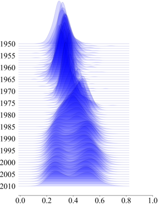
Source: Voth and Yanagizawa-Drott (CEPR Working Paper 2024), Figure 9
To illustrate how to make a ridge plot, I take the data from “how good is ’good’”. We have a list of words, such as “great”, “perfect”, etc. For each word, we ask people to give a score from 0 to 10, where 10 means very good, and 0, very bad. In the end, the data we have look like
| Score | Good | Great | Perfect |
|---|---|---|---|
| 0 | 1 | 0 | 0 |
| 1 | 0 | 0 | 0 |
| 2 | 3 | 5 | 0 |
| … | … | … | … |
| 9 | 30 | 33 | 10 |
| 10 | 25 | 35 | 80 |
, where 25 means 25 people give a score of 10 for the word “good”.
For each word, we make a kernel density plot, and then arrange all the plots from top to bottom, i.e. put them in a 3-row 1-col. figure.

Notes: Data behind this figure is synthetic, not the original data from how good is "good"
The trick is then to reduce the vertical gaps between the subfigures, so visually the distribution overlaps with each other a bit. We can also fill the distribution with some semi-transparent colour, so that the figures look like 3D ish.

Source: YouGov Word Sentiment and YouGov Word Sentiment 2