Double/debiased machine learning
(Code available at harningle/useful-scripts)
A short informal and not rigorous note on double machine learning.
Why naïve machine learning is wrong
Setup
Suppose we have the following data generating process (DGP):
\[\begin{equation}y_i = \beta x_i + f(\vec{z_i}) + \varepsilon_i \label{eq:dgp}\end{equation}\], where $y$ is the outcome, $x$ is the explanatory variable, associated with the true parameter $\beta$. $\vec{z}$ is some control variable(s), and it comes into the model (in a potentially non-linear way) as $f(\cdot)$. $\varepsilon$ is the usual Gaussian noise. $\vec{z}$ and $x$ are of course correlated (otherwise we don’t need to control it in the first place):
\[\begin{equation}x_i = g(\vec{z_i}) + \xi_i \label{eq:g}\end{equation}\], where $\xi$ again has a standard normal distribution. An easy way to think about it is as follows. We want to study the treatment effect of aspirin on headache, and have collected a random sample from the population. For each person, we know whether she has taken an aspirin, whether her headache is gone afterwards, and we have her basic health info.:
- $i$: a person in our sample
- $y$: headache
- $x$: aspirin
- $\vec{z}$: body weight, blood pressure, etc.
- $y_i = \beta x_i + f(\vec{z_i}) + \varepsilon_i$ ($\ref{eq:dgp}$): aspirin has $\beta$ effect on headache, and things like blood pressure can also impact headache in $f(\cdot)$ way
- $x_i = g(\vec{z_i}) + \xi_i$ ($\ref{eq:g}$): whether or not you take a pill partially depends on your health conditions in $g(\cdot)$ way
How to use ML
Non-Linearity Is the Problem. The textbook econometrics would simply control $\vec{z}$, like $y_i = \beta x_i + \delta_1 z_{1, i} + \delta_2 z_{2, i} + \cdots + \varepsilon_i$. The problem is that it only controls the linear relationship between $x$ and $\vec{z}$, but the nonlinear correlation between them is still there, and biases our estimate.
ML to Estimate This Non-Linearity. In order to capture such nonlinear relationship, a straightforward and naïve way is to use some machine learning method to fit $f(\cdot)$, plug the estimated $\hat f(\cdot)$ into the model, and run the regression as usual. In order to get a unbiased estimate of $\beta$, $x$ and $\varepsilon$ has to be uncorrelated, i.e.
\[\text{E}(x\varepsilon) = 0 = \text{E}\big (x({\color{blue}y - \beta x - f(\vec{z})})\big )\]. So far nothing is mathematically wrong. Now suppose we have some machine learning model estimate of $\hat f(\cdot)$, and we plug this to replace $f(\cdot)$ in the above moment condition:
\[\text{E}(x\varepsilon) = \text{E}\big (x({\color{blue}y - \beta x - {\color{red}\hat f(\vec{z})}})\big ) = 0\]ML brings problems
ML Introduces Bias. The ML estimation of course can’t be perfect, so it has certain prediction/estimation error $\eta$:
\[f(\vec{z}) = {\color{red}\hat f(\vec{z}) + \eta}\]. Now after plugging the estimated model, the new moment becomes
\[\begin{aligned} \text{E}(x\varepsilon) &= \text{E}\big (x({\color{blue}y - \beta x - f(\vec{z})} - {\color{red}\eta})\big ) \\ &= \text{E}\big (x({\color{blue}y - \beta x - f(\vec{z}})\big ) - \text{E}(x{\color{red}\eta}) \\ &= 0 - \text{E}(x{\color{red}\eta}) \\ &= -\text{E}(x{\color{red}\eta}) \end{aligned}\]. Compared with the original moment condition, we have one additional term $-\text{E}(x{\color{red}\eta})$. We have no reason whatsoever to say our explanatory variable $x$ has no relationship with ML model estimation error $\eta$. So generally we have a non-zero bias term here.
We May Still Have Consistency. Biases may still be OK-ish. IV is also biased, but we still use IV, because it is consistent. Can this be consistent as well? Empirically, The moment condition implies
\[\frac{1}{n}\sum\limits_{i = 1}^n x_i\big (y_i - \beta x_i - {\color{red}\hat f(\vec{z_i})}\big ) = 0\], or
\[\begin{aligned} \hat\beta &= \frac{\frac{1}{n}\sum\limits_i x_i(y_i - {\color{red}\hat f(\vec{z_i})})}{\frac{1}{n}\sum\limits_i x_i^2} \\ &= \frac{\frac{1}{n}\sum\limits_i x_i(y_i - f(\vec{z_i}) + {\color{red}\eta_i})}{\frac{1}{n}\sum\limits_i x_i^2} \\ &= \frac{\frac{1}{n}\sum\limits_i x_i(\overset{\text{Plug in (}\ref{eq:dgp}\text{)}}{\overbrace{y_i}} - f(\vec{z_i}))}{\frac{1}{n}\sum\limits_i x_i^2} + \frac{\frac{1}{n}\sum\limits_i x_i{\color{red}\eta_i}}{\frac{1}{n}\sum\limits_i x_i^2} \\ &= \frac{\frac{1}{n}\sum\limits_i x_i(\beta x_i + f(\vec{z_i}) + \varepsilon_i - f(\vec{z_i}))}{\frac{1}{n}\sum\limits_i x_i^2} + \frac{\frac{1}{n}\sum\limits_i x_i{\color{red}\eta_i}}{\frac{1}{n}\sum\limits_i x_i^2} \\ &= \frac{\frac{1}{n}\sum\limits_i x_i(\beta x_i + \varepsilon_i)}{\frac{1}{n}\sum\limits_i x_i^2} + \frac{\frac{1}{n}\sum\limits_i x_i{\color{red}\eta_i}}{\frac{1}{n}\sum\limits_i x_i^2} \\ &= \beta + \frac{\frac{1}{n}\sum\limits_i x_i\varepsilon_i}{\frac{1}{n}\sum\limits_i x_i^2} + \frac{\frac{1}{n}\sum\limits_i x_i{\color{red}\eta_i}}{\frac{1}{n}\sum\limits_i x_i^2} \end{aligned}\]. The probability limit is then
\[\DeclareMathOperator*{\plim}{plim} \plim\limits_{n\to\infty}\hat\beta - \beta = \frac{\plim\limits_{n\to\infty}\frac{1}{n}\sum\limits_i x_i\varepsilon_i}{\frac{1}{n}\sum\limits_i x_i^2} + \frac{\plim\limits_{n\to\infty}\frac{1}{n}\sum\limits_i x_i{\color{red}\eta_i}}{\frac{1}{n}\sum\limits_i x_i^2}\]. Law of large numbers guarantees the usual sampling error has $\plim\limits_{n\to\infty}\frac{1}{n}\sum\limits_i x_i\varepsilon_i = \text{E}(x\varepsilon)$ equalling zero, so
\[\plim\limits_{n\to\infty}\hat\beta - \beta = \frac{\plim\limits_{n\to\infty}\frac{1}{n}\sum\limits_i x_i{\color{red}\eta_i}}{\frac{1}{n}\sum\limits_i x_i^2}\]. We apply Cauchy-Schwarz inequality to the second term:
\[\begin{equation}\plim\limits_{n\to\infty}\frac{1}{n}\sum\limits_i x_i{\color{red}\eta_i} \leq \plim\limits_{n\to\infty}\sqrt{\frac{1}{n}\sum\limits_i x_i^2}\cdot\sqrt{\frac{1}{n}\sum\limits_i {\color{red}\eta_i}^2} \label{eq:cs}\end{equation}\]. The first term is a constant, so $O_p(1)$, and the second term is basically how fast the ML estimation converges to the true model; let’s call it $O_p(r)$. So as long as the ML model converges at all (slowly or quickly), e.g. $O_p(r) = O_p(n^{-0.005})$, the second term is zero as well:
\[\plim\limits_{n\to\infty}\frac{1}{n}\sum\limits_i x_i{\color{red}\eta_i} \leq O_p(1)\cdot \underset{\text{assume convergence}}{\underbrace{O_p(r)}} = 0\]. Therefore, if we have a reasonably good ML model whose estimation converges to the true model, the estimated coefficient is consistent:
\[\plim\limits_{n\to\infty}\hat\beta - \beta = 0\]. So just like IV, it’s biased, but with a good ML model, it’s still consistent.
Asymptotic Normality Is Gone, Always. Even if it’s consistent, the asymptotic distribution is not necessarily normal. To see it, scale it by root $n$:
\[\begin{aligned} \sqrt n(\hat\beta - \beta) &= \underset{\text{CLT gives normality for the usual error}}{\underbrace{\sqrt n \frac{\frac{1}{n}\sum\limits_i x_i\varepsilon_i}{\frac{1}{n}\sum\limits_i x_i^2}}} + \sqrt n\frac{\frac{1}{n}\sum\limits_i x_i{\color{red}\eta_i}}{\frac{1}{n}\sum\limits_i x_i^2} \\ &= O_p(n^{-\frac{1}{2}}) + O_p(r) \\ &= O_p \big (\max(n^{-\frac{1}{2}}, r)\big ) \end{aligned}\]. I’d like to elaborate the second term. $\text{E}(x\eta)$ may or may not be zero, but we can always use CLT:
\[\sqrt n\frac{1}{n}\sum\limits_i x_i{\color{red}\eta_i} \overset{d}{\to} \mathcal{N}\big (\text{E}(x\eta), \text{Var}(x\eta)\big )\]. So the second term does converge at usual CLT speed $O_p(n^{-\frac{1}{2}})$. However, it doesn’t converge to zero; it goes to $\text{E}(x\eta)$ instead. $\text{E}(x\eta)$ is not zero but $O_p(r)$. So whenever $O_p(r)$ is slower than $O_p(n^{-\frac{1}{2}})$, the estimator can’t be root-$n$ consistent, and will not have a valid asymptotic normal distribution. In reality, this is often true: a usual linear regression converges (much) faster than a complicated machine learning model, and the slowness of convergence of the ML model causes the second term to explode. Without asymptotic normality, we can’t have valid standard errors or do hypothesis testing. This is a big problem.
Frisch-Waugh-Lovell is the fix
Intuition
A natural question to ask is, why IV is also biased but it still keeps all nice asymptotic properties, but the naïve ML here is biased but has no valid asymptotic normal distribution.
| Naïve ML | IV | |
|---|---|---|
| First stage | Estimate relationship between $x$ and the control $z$, $f(\cdot)$ | Estimate relationship between $x$ and IV $z$, and get the residuals |
| Second stage | Plug the estimated relationship $\hat f(\cdot)$ into original regression | Replace $x$ with the residuals from the first stage in the original regression |
| Biased | Yes | Yes |
| Consistent | Maybe yes | Yes |
| Asymptotic Normal | No | Yes |
The key here is really the residuals: $x$ has a “clean” exogenous component and a “dirty” endogenous component, which is correlated with the control $z$. Rather than modelling this “dirty” correlation and control it, we can simply partial out the “dirty” component, and only uses the “clean” part:
\[x_i = \underset{\text{“dirty"}}{\underbrace{g(\vec{z_i})}} + \underset{\text{“clean"}}{\underbrace{\text{whatever left}_i}}\]. Similarly, we take the “dirty” part away from the outcome $y$ as well:
\[y_i = \underset{\text{“dirty"}}{\underbrace{l(\vec{z_i})}} + \underset{\text{“clean"}}{\underbrace{\text{whatever left}_i}}\]We can thus use whatever fancy ML methods to extract the “dirty” part away from $x$ and $y$, and then a residuals-on-residuals regression will give
\[\text{“clean" part of }y_i = \beta\text{“clean" part of }x_i + \zeta_i\]. This is precisely the same intuition as Frisch-Waugh-Lovell theorem, but in a slightly complicated/non-linear way.
The estimator
Is the above intuition correct? Frisch-Waugh-Lovell theorem is valid for linear regressions, but here $g(\cdot)$ and $l(\cdot)$ are not necessarily linear. Let’s check what exactly we get from this residuals-on-residuals regression. First, we use whatever ML model(s) to estimate $\hat g(\cdot)$ and $\hat l(\cdot)$, and then obtain the residuals:
\[\begin{align} \tilde x_i &= x_i - {\color{orange}\hat g(z_i)} \label{eq:tilde_x} \\ \tilde y_i &= y_i - {\color{purple}\hat l(z_i)} \label{eq:tilde_y} \\ \end{align}\]. Then the OLS coefficient of regressing $\tilde y_i$ on $\tilde x_i$ is the usual
\[\begin{equation}\hat\beta = \frac{\frac{1}{n}\sum\limits_i\tilde y_i \tilde x_i}{\frac{1}{n}\sum\limits_i\tilde x_i^2} \label{eq:beta_hat}\end{equation}\]. Suppose the ML estimation errors for $\hat g(\cdot)$ and $\hat l(\cdot)$ are $u$ and $v$:
\[\begin{align} g(z_i) &= {\color{orange}\hat g(z_i)} + u_i \label{eq:u} \\ l(z_i) &= {\color{purple}\hat l(z_i)} + v_i \label{eq:v} \\ \end{align}\]. Plug ($\ref{eq:tilde_x}$), ($\ref{eq:tilde_y}$), ($\ref{eq:u}$), and ($\ref{eq:v}$) into ($\ref{eq:beta_hat}$), and let’s focus on the numerator now.
\[\begin{aligned} \frac{1}{n}\sum\limits_i\tilde y_i \tilde x_i &= \frac{1}{n}\sum\limits_i \big (y_i {\color{purple}- l(z_i) + v_i}\big ) \big (x_i {\color{orange}- g(z_i) + u_i}\big )\\ &= \frac{1}{n}\sum\limits_i \big (\beta x_i + f(\vec{z_i}) + \varepsilon_i -{\color{purple} l(z_i) + v_i}\big ) \big (x_i {\color{orange}- g(z_i) + u_i}\big ) \end{aligned}\].Here $l(\cdot)$ and $g(\cdot)$ are the goals of ML model estimations, and the only “ML-unrelated” thing is $f(\vec{z})$. So let’s try to eliminate it. We know $l(\vec{z})$ is the relationship between $y$ and $\vec{z}$, which, by definition, means
\[\begin{equation}{\color{purple}l(\vec{z})} = {\color{purple}\text{E}(y | \vec{z})} \label{eq:l_cond_mean}\end{equation}\]. For the same reason, $g(\vec{z})$ is also a conditional mean:
\[\begin{equation}{\color{orange}g(\vec{z})} = {\color{orange}\text{E}(x | \vec{z})} \label{eq:g_cond_mean}\end{equation}\]And taking the expectation on both sides of DGP ($\ref{eq:dgp}$) gives
\[\begin{equation}{\color{purple}\text{E}(y | \vec{z})} = \beta {\color{orange}\text{E}(x | \vec{z})} + f(\vec{z}) + \text{E}(\varepsilon | \vec{z}) = \beta {\color{orange}\text{E}(x | \vec{z})} + f(\vec{z}) + 0 \label{eq:y_cond_mean}\end{equation}\]. Combining ($\ref{eq:l_cond_mean}$), ($\ref{eq:g_cond_mean}$), and ($\ref{eq:y_cond_mean}$), we have
\[\begin{equation}{\color{purple}l(\vec{z})} = {\color{purple}\text{E}(y | \vec{z})} = \beta {\color{orange}g(\vec{z})} + f(\vec{z})\label{eq:l_g_f}\end{equation}\]Now plugging ($\ref{eq:l_g_f}$) into $\displaystyle \frac{1}{n}\sum\limits_i\tilde y_i \tilde x_i$, we have a simplified numerator:
\[\begin{aligned} \frac{1}{n}\sum\limits_i\tilde y_i \tilde x_i &= \frac{1}{n}\sum\limits_i \big (\beta x_i + f(\vec{z_i}) + \varepsilon_i -{\color{purple} l(z_i) + v_i}\big ) \big (x_i {\color{orange}- g(z_i) + u_i}\big ) \\ &= \frac{1}{n}\sum\limits_i \big (\beta x_i + \overset{f(\vec{z_i})}{\overbrace{ {\color{purple}l(\vec{z_i})} - \beta{\color{orange}g(\vec{z_i})}}} + \varepsilon_i - {\color{purple} l(z_i) + v_i}\big ) \big (\xi_i + {\color{orange}u_i}\big ) \\ &= \frac{1}{n}\sum\limits_i \big (\beta x_i - \beta{\color{orange}g(\vec{z_i})} + \varepsilon_i + {\color{purple} v_i}\big ) \big (x_i {\color{orange}- g(z_i) + u_i}\big ) \\ &= \frac{1}{n}\sum\limits_i (\beta \xi_i + \varepsilon_i + {\color{purple} v_i})(\xi_i + {\color{orange}u_i}) \end{aligned}\]. There are six terms in total:
- $\text{E}(\beta\xi^2) = \beta\text{Var}(\xi) = \beta$ because $\xi$ is standard normal by construction and thus has unit variance
- $\text{E}(\beta\xi {\color{orange}u}) = \beta\text{E}(\xi {\color{orange}u}) = \beta\cdot 0 = 0$. $\xi$ and $\color{orange}u$ are not correlated, because $\xi$ is not correlated with $\vec{z}$ by zero conditional mean, and $\color{orange}u$ is purely a function of $\vec{z}$ only, as it’s the prediction/estimation error of a function of only $\vec{z}$
- $\text{E}(\varepsilon\xi) = 0$ by construction of DGP (zero conditional mean again)
- $\text{E}(\varepsilon {\color{orange}u}) = 0$ for the same reason as 2.
- $\text{E}({\color{purple} v}\xi) = 0$ for the same reason as 2.
- $\text{E}({\color{purple} v}{\color{orange}u})$: a second order term1
Cross fitting
One subtlety above is “$\color{orange}u$ is purely a function of $\vec{z}$ only, as it’s the prediction/estimation error of a function of only $\vec{z}$”. This is not always true. $\color{orange}u$ is the model prediction error, and the model is trained on the sample, so of course $\color{orange}u$ is a function of the training set. $\xi$ is the noise in DGP, so the data points, or the outcome to be more precise, in the training set contain this noise. In this sense, $\color{orange}u$ and $\xi$ can well be correlated due to the shared/common noise in the sample.
The fix is fortunately straightforward: since the cause is the noise appears in the model prediction error and the outcome in the data points at the same time, we can train the model somewhere else, and make sure the training never sees outcomes when we estimate the coefficient. E.g., we have ten data points, shuffle them, and use the first five to estimate $\hat g(\cdot)$ and $\hat l(\cdot)$. Then we run the residuals-on-residuals regression on the other five data points. For observation 6, it has the usual residual $\tilde x_6 = x_6 - \hat g(\vec{z_6}) = x_6 - {\color{orange}g(\vec{z_6}) + u_6} = \xi_6 + {\color{orange}u_6}$. Here $\xi_6$ is the noise in DGP; we can’t do anything. $\color{orange}u_6$ is the model prediction error. Our ML model $\hat g(\cdot)$ is now trained on sample 1 to 5. So yes, it is still correlated with $\varepsilon$ and $\xi$, but this correlation solely depends on $\varepsilon_1, \cdots, \varepsilon_5, \xi_1, \cdots, \xi_5$. It has absolutely zero relationship with $\varepsilon_6$ or $\xi_6$! Therefore, with cross fitting, we can safely say $\text{E}(\varepsilon\xi)$ and $\text{E}(\varepsilon u)$ are zero.
The denominator is
\[\begin{aligned} \frac{1}{n}\sum\limits_i\tilde x_i^2 &= \frac{1}{n}\sum\limits_i \big (x_i - \underset{\text{Plug in (}\ref{eq:u}\text{)}}{\underbrace{\hat g(\vec{z_i})}} \big )^2 \\ &= \frac{1}{n}\sum\limits_i \big (\underset{\text{Plug in (}\ref{eq:g}\text{)}}{\underbrace{x_i}} - g(\vec{z_i}) + u_i \big )^2 \\ &= \frac{1}{n}\sum\limits_i (\xi_i + u_i)^2 \\ &= \frac{1}{n}\sum\limits_i (\xi_i^2 + \xi_i u_i + u_i^2) \end{aligned}\]. The three terms are very similar to the terms in the numerator:
- $\text{E}(\xi^2)$ is the variance of $\xi$, which is 1 by construction
- $\xi$ and $u$ are not correlated, so $\text{E}(\xi u)$ is zero
- $\text{E}(u^2) = \text{Var}(u)$ and it is what it is
It’s still biased
Unfortunately (and maybe expectedly), the estimator is biased.
\[\begin{aligned} \text{E}(\hat\beta) &= \frac{\beta + \text{E}\Big (\frac{1}{n}\sum\limits_i {\color{purple}v_i}{\color{orange}u_i} \Big )}{1 + \text{E}\Big (\frac{1}{n}\sum\limits_i {\color{orange}u_i}^2 \Big )} \\ &= \frac{\beta + \text{E}(uv)}{1 + \text{Var}(u)} \\ &\approx \beta + \text{E}(uv) \big (1 - \text{Var}(u) \big ) \end{aligned}\]The last line uses binomial approximation that $(1 + x)^n = 1 + nx + o(x)$ when $x$ is sufficiently small, and yes, we assume $\text{Var}(u)$ is very small. Generally this is not unbiased, because we have no guarantee that the terms after $\beta$ are zero.
Consistency
The probability limit of the estimator is
\[\begin{aligned} \plim\limits_{n\to\infty} \hat\beta &= \frac{\beta + \plim\Big (\frac{1}{n}\sum\limits_i u_i v_i \big )}{1 + \plim\Big (\frac{1}{n}\sum\limits_i u_i^2 \Big )} \\ &= \frac{\beta + \text{E}(uv)}{1 + \text{Var}(u)} \\ &\approx \frac{\beta + \sqrt{\text{Var}(u)}\sqrt{\text{Var}(v)}}{1 + \text{Var}(u)} \end{aligned}\]. Here we use the Cauchy-Schwarz inequality as in ($\ref{eq:cs}$) again. So as long as ML models $\hat g(\cdot)$ and $\hat l(\cdot)$ are reasonably good, all those variances are going to zero when we have an infinitely big sample, and then $\plim \hat\beta = \beta$. We do have consistency.
Asymptotic normality
Recall that we have six terms in the numerator and three terms in the denominator. Out of nine, four are linear in the model prediction error: $\displaystyle\frac{1}{n}\sum\limits_i\xi_i u_i$, $\displaystyle\frac{1}{n}\sum\limits_i\xi_i v_i$, $\displaystyle\frac{1}{n}\sum\limits_i\varepsilon_i u_i$, and $\displaystyle\frac{1}{n}\sum\limits_i \xi u_i$. Basically they are the model prediction error (like a constant) interacted with the Gaussian noise in DGP.2 So all of them have an expected value of zero, and CLT gives nice results.
Furthermore, there are two second order terms: $\displaystyle\frac{1}{n}\sum\limits_i u_i^2$ in the denominator and $\displaystyle\frac{1}{n}\sum\limits_i u_i v_i$ in the numerator. For simplicity, let’s assume both $\hat g(\cdot)$ and $\hat l(\cdot)$ converge at the speed of $o_p(r)$. Then both second order terms are $O_p(r^2)$. Therefore,
\[\hat\beta = \frac{\beta\frac{1}{n}\xi_i^2 + \overset{\text{usual CLT}}{\overbrace{\frac{1}{n}\sum\limits_i\xi_i\varepsilon_i}} + \overset{\text{three first order term}}{\overbrace{o_p(n^{-\frac{1}{2}}) + o_p(n^{-\frac{1}{2}}) + o_p(n^{-\frac{1}{2}})}} + \overset{uv}{\overbrace{O_p(r^2)}}}{\underset{\text{unit variance by construction}}{\underbrace{\sum\limits_i\frac{1}{n}\xi_i^2}} + \underset{u^2}{\underbrace{O_p(r^2)}} + \underset{\text{another first order term}}{\underbrace{o_p(n^{-\frac{1}{2}})}}}\]. Therefore,
\[\begin{aligned} \sqrt{n} (\hat\beta - \beta) &= \frac{1}{\sqrt{n}}\sum\limits_i\xi_i\varepsilon_i + \sqrt{n} O_p(r^2) + o_p(1) \\ &= O_p(n^{-\frac{1}{2}}) + O_p(r^2) \end{aligned}\].3 Now so as to have nice asymptotic property, $O_p(r^2)$ needs to be at least as fast as $O_p(n^{-\frac{1}{2}})$, which means $r^2 \leq n^{-\frac{1}{2}}$, or $r \leq n^{-\frac{1}{4}}$. This indicates that as long as the ML models converge faster than $n^{-\frac{1}{4}}$, we will have a valid asymptotic normal distribution.
What orthogonalisation and cross fitting bring us
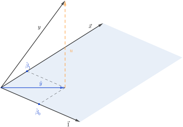
Residual Is Orthogonal to the Fitted Value. I believe this deserves a separate discussion. Frisch-Waugh-Lovell theorem is basically a residuals-on-residuals regression, which aims at using the “clean” component to identify the coefficient by partialling out the “dirty” variation. Why we call this “orthogonalisation”? Recall the simplest univariate regression:
\[\begin{aligned} y &= \beta_0 + \beta_1 x + \varepsilon \\ \hat y &= \hat\beta_0 + \hat\beta_1 x \\ y &= \hat y + u \end{aligned}\]. Here the prediction error, or the residual, is $u$. And $u$ must be orthogonal to $\hat y$. You can see this easily from the normal equation, or from the visualisation below. The intuition is straightforward: we try our best to explain $y$ using $x$’s, and our prediction/fitted value is always on the subspace spanned by $x$’s, and the residual is thus perpendicular to this subspace. This is why we call the residuals “orthogonalisation”.
Cross Fitting Kills First Order Terms. We have a short discussion about cross fitting above, and I want to re-iterate the key idea. When we brute force the estimator, we get terms like $\xi \color{orange}u$, where $\xi$ is the noise in DGP, and $\color{orange}u$ is the prediction error. There is generally no analytical guarantee that such terms like $\xi \color{orange}u$ have a mean of zero. If anything, we have some reason to believe $\xi$ and $\color{orange}u$ are correlated: $\color{orange}u$ is the model prediction error, so surely $\color{orange}u$ depends on the model. The model is trained on the sample, so $\color{orange}u$ also depends on the sample. The sample is generated from DGP, which has noise $\xi$, so $\color{orange}u$ may also depend on $\xi$.4 Consequently, these first order terms have a non-zero probability limit, and will invalidate the asymptotic distribution. Cross fitting means we train the model on a subset of the sample, and then do regression using the rest of the sample. By doing so, no matter how $\color{orange}u$ is correlated with the noise, such correlation is limited to the correlation with the noise in the training set. Data points are i.i.d., so these noises are independent of the noise in the estimation set. In short, $\color{orange}u$ only depends on the training set, and $\xi$ is the noise in the rest of the data, so they can’t be correlated. Therefore, all such first order terms become zero if we cross fit.
No First Order Terms Imply Zero Asymptotic Average. Thanks to cross fitting, all first order terms converge to zero, and we are left with second order terms only, i.e. $\xi\varepsilon$, $uv$, and $u^2$. $\xi\varepsilon$ are the multiplication of two Gaussian noises by construction, so CLT handles it easily, and convergence speed is no problem. $uv$ and $u^2$ are the second order terms of model prediction errors. We can assume models are good so they converge to zero.
If Have Second Order Terms Only, Can Afford Slower Convergence, Relative to the Naïve Way. The remaining problem is the rate: do they go to zero fast enough? $\xi\varepsilon$ for sure due to CLT. Then the bottleneck is the two second order terms. The naïve ML way has its convergence rate depending on a first order term of model prediction error $x\eta$. Here after using Frisch-Waugh-Lovell theorem, the convergence rate is a second order term of model prediction error! So it was $O_p(r)$ but now it is $O_p(r^2)$! As a result, we can allow for slower convergence of the ML models, as long as they are faster than $O_p(n^{-\frac{1}{4}})$.
Simulation
Now let’s run a toy simulation to see if any of the above math actually shows up in the data.
The DGP
We keep ($\ref{eq:dgp}$) and ($\ref{eq:g}$), so all that’s left is to pick $f(\cdot)$ and $g(\cdot)$. Back to the aspirin story: for each of the $n = 1{,}000$ persons in the sample, we observe ten health indicators $z_1, \cdots, z_{10}$, all i.i.d. standard normal. Every one of them affects the headache, in the same wiggly way, but only the first affects whether a person takes a pill:
\[\begin{aligned} f(\vec z) &= \sin(z_1) + \cdots + \sin(z_{10}) \\ g(\vec z) &= \sin (z_1) \end{aligned}\], and everything else is as assumed above: both $\varepsilon$ and $\xi\sim\mathcal{N}(0, 1)$, and aspirin works with a coefficient $\beta = 0.5$.
We don’t know the exact functional form of $f(\cdot)$ or $g(\cdot)$: we don’t know which of the ten health indicators matter, nor that they enter as sines. So we just hand everything to a machine learning model and let the model work out $f$, $g$, and $l$. For simplicity, we use gradient boost machine with default hyperparameters from scikit-learn.5
from sklearn.ensemble import GradientBoostingRegressor

GradientBoostingRegressor(random_state=seed).fit(inputs, target).predict(pred)
The estimators
We run the following on each of 1,000 data points sampled from the above DGP.
Oracle. Residualise using the true $\color{orange}g(\cdot)$ and $\color{purple}l(\cdot)$, i.e. ($\ref{eq:beta_hat}$) with no ML anywhere. Infeasible, but it tells us how much sampling noise is irreducible.
OLS. $y_i = \alpha + \beta x_i + \vec\delta^T\vec{z_i} + \text{error}$, the textbook approach we started from.
Naïve. The moment condition from above is
\[\hat\beta = \frac{\sum\limits_i x_i\big (y_i - {\color{red}\hat f(\vec{z_i})}\big )}{\sum\limits_i x_i^2}\]. There is a practical annoyance: unlike $\color{purple}l$ and $\color{orange}g$, $f$ is not the conditional mean of anything we observe, so there is nothing we can regress on $\vec z$ to get $\color{red}\hat f$ directly. We need a first guess of $\beta$ to build a target $y - \beta x$, and the OLS estimate above is what one would reach for. Then $\color{red}\hat f$ is fitted on the whole sample and plugged straight back in. That is, use an ML model to predict $y - \hat\beta_{OLS}x$ using $\color{red}\vec z$, and then plug this model $\color{red}\hat f(\vec z)$ into the original DGP and get $\hat\beta$ using a normal OLS regression. 6
Orthogonalised, Without cross Fitting. Fit $\color{purple}\hat l$ and $\color{orange}\hat g$ using all data points, take the residuals ($\ref{eq:tilde_x}$), and ($\ref{eq:tilde_y}$), and run the residuals-on-residuals regression ($\ref{eq:beta_hat}$).
DDML. The same as above, except $\color{purple}\hat l$ and $\color{orange}\hat g$ are 5-fold cross fitted: we randomly divide the whole dataset into five equal-sized fold, and then for each fold, the ML model is trained on the other four folds, and predicts and take the residuals on the holdout one, and finally the residuals-on-residuals regression is also run on this holdout fold.7
Results

(A) Naïve ML

(B) Orthogonalised, w/o cross fitting

(C) DDML
Notes: Histograms are the simulated distribution of $\frac{\hat\beta - \beta}{\widehat{\text{s.e.}}}$ over 1,000 replications, and the red line is the standard normal density. Coverage is the share of replications whose 95% confidence interval covers the true $\beta = 0.5$. All three panels share the same axes, so they can be compared directly. The range covers the 1st to 99th percentile of every estimator, which clips 0.9% of the naïve estimator's right tail into the last bin.
| Estimator | Bias | Avg. s.e. | 95% coverage |
|---|---|---|---|
| Oracle | +0.001 | 0.032 | 95.6% |
| OLS | +0.060 | 0.040 | 69.0% |
| Naïve ML | +0.055 | 0.019 | 29.3% |
| No cross fitting | -0.100 | 0.030 | 9.4% |
| DDML | -0.010 | 0.038 | 94.2% |
DDML Works. Bottom line first: DDML lands on the standard normal: bias -0.010 against the oracle’s +0.001, and 94.2% coverage against the oracle’s 95.6% and a nominal 95%. It does have larger s.e. compared to the oracle, of course, as we use ML models to estimate $l$ and $g$.
The Naïve ML Is an Expensive Way to Re-Run OLS. It is off by 0.055 and covers the truth 29.3% of the time, which is bad enough. To some degree, this is not surprising: we start from an initial guess of $\beta$ and then hope, by using ML, we get a more accurate estimate. This can happen in many cases, e.g. two-step feasible GMM, but it’s not the case here. See discussion here. The short answer is that ML models have their own errors, which isn’t going away during the iterations, so the estimator can’t converge to its fixed point (the true $\beta$).
And It Doesn’t Know It. There is a second (more subtle but important) failure stacked on the first. The reported standard error is 0.019, while the actual spread of $\hat\beta$ across replications is 0.036, so it’s understated by a factor of two. The in-sample residuals $y - \color{red}\hat f$ are artificially small, so the final regression looks twice as precise as it really is. Biased and overconfident, which is why coverage collapses to 29.3% rather than the ~60% the bias alone would cost. It is visible in the left panel of the figure: that histogram is not merely shifted, it is wider than the normal curve. A correctly calibrated $t$ value should have unit variance, while this one is spread over roughly twice that. Nothing on the printout looks wrong: the point estimate is plausible, the standard error is tight, and the stars are there, but it’s in fact wrong.
Why the Same Model Is Fine Inside DDML. Because the two estimators lean on the ML error in completely different ways. The cross fitted $\color{orange}\hat g$ misses $\color{orange}g$ by 0.315 in root mean square, while $\color{purple}\hat l$ misses $\color{purple}l$ by 0.745.8 The naïve bias is first order in the outcome side error, so that 0.745 walks straight into $\hat\beta$. The DDML bias instead runs through $\text{E}({\color{orange}u}{\color{purple}v})$, which the Cauchy-Schwarz inequality ($\ref{eq:cs}$) caps at 0.315 × 0.745 = 0.235, and which actually comes out at 0.037, because the two errors are nowhere near parallel. This is the $O_p(r)$ versus $O_p(r^2)$ contrast from above. The outcome equation is a ten dimensional problem and the model does poorly on it; the treatment equation is a one dimensional problem and the model does well on it. DDML never has to be good at both. It only needs to avoid being bad at both at once, a far weaker thing to ask for.
Cross Fitting Is Not Optional. The whole argument for cross fitting was that $\text{E}(\xi{\color{orange}u})$ and other terms are not zero when the model is trained on the very rows we then residualise. We can simply measure it:
| $\overline{\xi{\color{orange}u}}$ | $\overline{ {\color{orange}u}^2}$ | $\frac{1}{n}\sum_i \tilde x_i^2$ | |
|---|---|---|---|
| W/o cross fitting | -0.261 | 0.124 | 0.602 |
| Cross fitted | -0.001 | 0.100 | 1.098 |
| Ideal | close to 0 due to cross fitting | very small if the ML model is good | slightly bigger than 1 since it’s unit variance plus $\text{E}({\color{orange}u}^2)$ |
Cross fitting does exactly what it says on the tin: $\overline{\xi{\color{orange}u}}$ lands on -0.001, zero to all intents and purposes. Without it the booster is contaminated: fitted on the very rows it then predicts, $\color{orange}\hat g$ has quietly absorbed a chunk of $\xi$, and $\overline{\xi{\color{orange}u}}$ comes out at -0.261 instead. Feed that into the denominator we derived above, and we get 0.602, against 1.098 when cross fitting. Nearly half of the variation that identifies $\beta$ has been eaten by the first stage before the second stage ever sees it. The result is a bias of -0.100, three times the oracle’s entire standard deviation, and a confidence interval that covers the truth 9.4% of the time.
And again the standard error does not warn us. It shrinks, from 0.038 to 0.030. The residuals got smaller, so the regression looks more precise, exactly while it becomes badly wrong. That is the second time in this table that a broken estimator has reported a tighter confidence interval than the working one.
The Two Shortcuts Fail for Opposite Reasons. The naïve approach dies of the model’s prediction error: it cannot pin down $f$, and that error enters at first order. Dropping cross fitting dies of the opposite problem, the model fitting its training rows too well and eating the very variation that identifies $\beta$. Orthogonalisation deals with the ML model being wrong, and cross fitting deals with it being wrong about the rows we are about to use. Separate fixes for separate diseases, and the right-hand panel is what you get only by applying both.
-
We mess up expectation, probability limit, and the average and the entire math here is very sloppy. See Chernozhukov et al. (Econometrics J. 2018) for a formal derivation. ↩
-
This “like a constant” is not trivial. CLT says a pure Gaussian noise converges nicely, and it’s trivial that 3× or 6× or whatever constant times this noise also converges nicely. However, what we have now is $u\times$ or $v\times$ the noise. Why the same convergence rate? All goes to cross fitting! We train ML models on a subset of our data, and then on the rest of the data we run the residuals-on-residuals regression to estimate the coefficient. This way, the model prediction errors, which is correlated with the noise in the training set, are independent of the noise in the estimation set. Therefore, $u\times$ the noise acts as if a constant times the noise, so the convergence rate is the same. ↩
-
The derivation here is not very solid. I replace terms in the denominator with their probability limit, so it’s $1 + 0 + 0$ and everything goes away. This is a sloppy application of Slutsky’s theorem. ↩
-
This is also generally wrong lol. Correlation doesn’t have transitivity. That is, if $\text{Corr}(X, Y) \neq 0$, and $\text{Corr}(Y, Z) \neq 0$, $\text{Corr}(X, Z)$ can take any value, zero or non-zero. It’s easy to construct examples. When $X = Y = Z$, $\text{Corr}(X, Y) = 1$, $\text{Corr}(Y, Z) = 1$, and $\text{Corr}(X, Z) = 1$ as well. When $X$ and $Z$ are i.i.d. normal and $Y = X + Z$, we have $\text{Cov}(X, Y) = \text{Cov}(X, X + Z)$. Using linearity, it is $\text{Var}(X) + \text{Cov}(X, Z) = 1 + 0 = 1$, $\text{Corr}(Y, Z)$ is 1 for the same reason. However, $\text{Cov}(X, Z) = 0$ by construction. See a very nice blog by Terrence Tao for more technical details. ↩
-
The simulation setup is not trivial. First, if DGP is simple enough, whatever models can then learn it easily, which means all model prediction errors are small (or even vanish), and models converge very quickly. This means even the naïve approach can give ok-ish result, because these first order error terms are tiny. Second, the ML models shouldn’t under- or overfit too much. If a model underfits, then all prediction errors are very big. In this case, the naïve approach fails due to the big first order terms. Second order terms are smaller in relative terms, but are still be big enough so that residuals-on-residuals regression won’t work either. If a model overfits, then two things can go wrong. One is that the prediction errors are huge and both first and second order terms are big, so nothing works. The other is specific to the non-cross fitting approach. If the model overfits severely, then the training loss is small or even close to zero. So all terms, in nominator or denominator, become tiny or zero, and the entire estimator degenerates to approx. $\frac{0}{0}$. The computer always gives a number, but we can’t trust it any more. Therefore, the DGP complexity and the ML model goodness of fit is really important here. The setup here happens to be on the sweet spot between overfitting and underfitting to demonstrate all approaches here. ↩
-
Expectedly, the initial guess of $\beta$ has a great impact on the final estimate. We use a simple OLS $\hat\beta_{OLS}$ here, which may or may not be a good guess. The official DoubleML docs. provides another (IMO better but slightly more complicated) way. This looks circular: we guess $\beta$, use the guess to learn $f$, then use $f$ to estimate $\beta$ again, so it’s worth pausing on why it isn’t. Suppose that $\color{red}\hat f$ were the exact conditional mean, i.e. $\color{red}\hat f = \text{E}(y - \hat\beta_{OLS} x \vert \vec z) = {\color{purple}l} - \hat\beta_{OLS}{\color{orange}g}$. Then $y - {\color{red}\hat f} = \beta\xi + \varepsilon + \hat\beta_{OLS}{\color{orange}g}$, and using $\text{E}(x\xi) = \text{Var}(\xi) = 1$ and $\text{E}(x{\color{orange}g}) = \text{Var}({\color{orange}g})$, the estimator returns $\hat\beta = \frac{\beta + \hat\beta_{OLS}\text{Var}({\color{orange}g})}{1 + \text{Var}({\color{orange}g})}$, or $\hat\beta - \beta = \frac{\text{Var}({\color{orange}g})}{1 + \text{Var}({\color{orange}g})}\big (\hat\beta_{OLS} - \beta\big )$. So the output is a weighted average of the truth and our guess, and the error shrinks rather than being passed through. It’s a contraction, and its fixed point is exactly $\beta$: iterate it and we converge on the truth wherever we start. What breaks it is that $\color{red}\hat f$ is often not that conditional mean, and it fails in two separate ways. The ML prediction error adds the $\text{E}(x{\color{red}\eta})$ term from above, which has nothing to do with our initial guess and therefore doesn’t shrink at all. And fitting $\color{red}\hat f$ on the whole sample destroys the contraction outright: if the model absorbs its own target completely, then $y - {\color{red}\hat f} = \hat\beta_{OLS}x$ and $\hat\beta = \hat\beta_{OLS}$ exactly, i.e. we get our guess handed straight back. Both of these happen below. ↩
-
Cross fitting also makes full use of the entire sample. One may think: I train the models on one part of the sample, and then run regression on the rest of the sample, so the regression only uses a subset of the dataset. Yes you can do it in this way; nothing wrong. But the following is better. Split the original dataset into two parts. Train the model in part 1, get residuals from part 2. The train the model in part 2, and get residuals from part 1. Now we have the residuals of part 1 and 2, i.e. the full sample, and can run residuals-on-residuals regression on the full sample. In the simulation we split the sample onto five parts, i.e. 5-fold cross fitting. ↩
-
Root mean squared error of the cross fitted predictions against the true nuisance function, averaged over 100 replications, as are all the numbers in the next table below. ↩