Lagrangian and KKT conditions
A quick recap of constrained optimisations.
Equality constraints
Geometrical intuition
Consider
\[\begin{aligned} &\min f(\vec{x}) \\ \text{s.t. } &h(\vec{x}) = 0 \end{aligned}\]. $f$ is a multivariate function of $\vec{x}$, and we can only pick $\vec{x}$ that is on the surface of $h(\vec{x}) = 0$. A concrete example would be
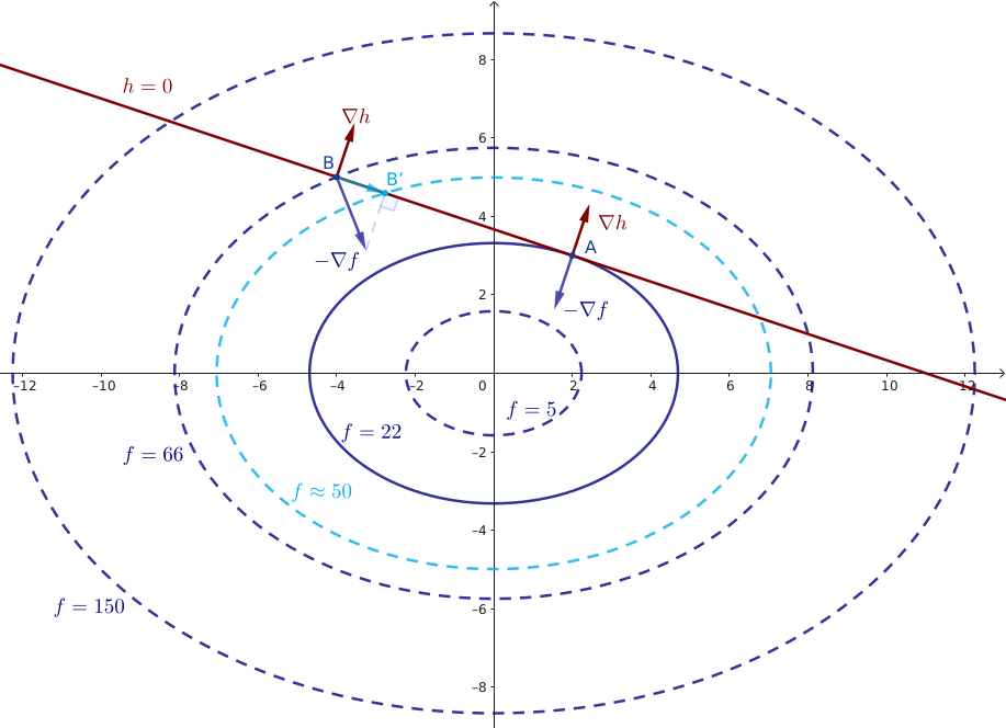
\[\begin{aligned} &\min f(x_1, x_2) = x_1^2 + 2x_2^2 \\ \text{s.t. } &h(x_1, x_2) = x_1 + 3x_2 - 11 = 0 \end{aligned}\]. So we try to pick some point on line $\color{maroon}h = 0$, and try to make the ellipse $\color{Blue}f$ as small as possible. The figure below plots a few contours of $\color{Blue}f$, and we pick the optimum point $\color{Blue}A$ and some other point $\color{Blue}B$ on the line. At the best point $\color{Blue}A$, $\color{Blue}\nabla f$ must be orthogonal to line $\color{maroon}h = 0$, or equivalently, parallel to $\color{maroon}\nabla h$. We can prove this by contradiction (in a sloppy way). Suppose $\color{Blue}B$ is the best point, and at that point the two gradients $\color{Blue}\nabla f$ and $\color{maroon}\nabla h$ are not parallel. By assumption, the projection of $\color{Blue}\nabla f$ onto line $\color{maroon}h = 0$ is not zero, because they are not perpendicular to each other. We can thus make a tiny move along the line in the direction of this projection $\color{Cerulean}\nabla f_{||h = 0}$. That is, move from $\color{Blue}B$ to $\color{Cerulean}B’$. $\color{Cerulean}B’$ satisfies the constraint because it’s still on the line, and such move would make $\color{Blue}f$ smaller, because we are moving in a direction that is some projection of the gradient $\color{Blue}\nabla f$. So $\color{Cerulean}B’$ is a better point than $\color{Blue}B$, which is a contradiction. Therefore, at optimum, two gradients must be parallel: ${\color{Blue}\nabla f} \parallel \color{maroon}\nabla h$.
The Lagrangian
More generally, at optimum $\vec{x}^*$, this parallel requirement translates to
\[\nabla f(\vec{x}^*) + \lambda\nabla h(\vec{x}^*) = 0\], for some $\lambda$. Now define the Lagrangian
\[\mathcal{L}(\vec{x}, \lambda) = f(\vec{x}) + \lambda h(\vec{x})\]. It’s a function of $\vec{x}$ and $\lambda$. One partial derivative/gradient
\[\frac{\partial\mathcal{L}}{\partial \vec{x}} = 0\]gives the parallel condition, and the other one
\[\frac{\partial\mathcal{L}}{\partial \lambda} = h\]gives back the constraint $h(\vec{x}) = 0$ when set to zero. So solving the unconstrained Lagrangian gives the solution.
In the above example, the Lagrangian is
\[\mathcal{L}(x_1, x_2, \lambda) = x_1^2 + 2x_2^2 + \lambda (x_1 + 3x_2 - 11)\]. Taking the derivatives:
\[\begin{aligned} \frac{\partial\mathcal{L}}{\partial x_1} &= 2x_1 + \lambda = 0 \\ \frac{\partial\mathcal{L}}{\partial x_2} &= 4x_2 + 3\lambda = 0 \\ \frac{\partial\mathcal{L}}{\partial \lambda} &= x_1 + 3x_2 - 11 = 0 \end{aligned}\]. And the solution is $x_1 = 2$ and $x_2 = 3$.
Inequality constraints
Inequality constraints are more difficult. Suppose we now have a constraint of $g(\vec{x})\leq 0$. The feasible set is a region rather than a line as in the equality case. There are two cases.
Optimum strictly inside the boundary
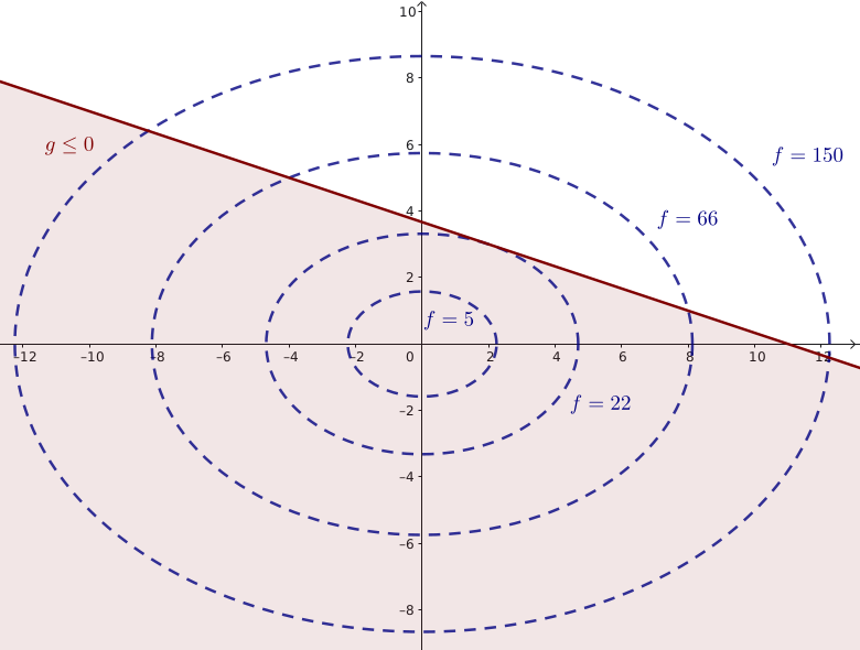
The first case is when the optimum is inside the boundary, i.e. $g(\vec{x}^*) < 0$. The constraint is then inactive and plays no role, so we can solve it as if it’s an unconstrained problem. Therefore, $\nabla f(\vec{x}^*) = 0$.
A numerical example would be
\[\begin{aligned} &\min f(x_1, x_2) = x_1^2 + 2x_2^2 \\ \text{s.t. } &g(x_1, x_2) = x_1 + 3x_2 - 11 \leq 0 \end{aligned}\]. It’s obvious that the global minimum is achieved when $x_1 = 0$ and $x_2 = 0$, and $(0, 0)$ satisfies $x_1 + 3x_2 - 11 = -11 < 0$.
Optimum is right on the boundary
The second case is when the optimum is right on the boundary, i.e. $g(\vec{x}^*) = 0$. The constraint is now active, and it’s like the equality case: optimum requires two gradients $\color{Blue}\nabla f$ and $\color{maroon}\nabla g$ to be parallel. But here we need to pay extra attention to direction. In subcase (A) below, point $A$ has $\color{Blue}\nabla f$ parallel to $\color{maroon}\nabla g$, and it’s the optimum. However, subcase (B) also has a point $A$ with $\color{Blue}\nabla f$ parallel to $\color{maroon}\nabla g$, but the real optimum happens at $(0, 0)$ (inside the feasible region) instead of point $A$.
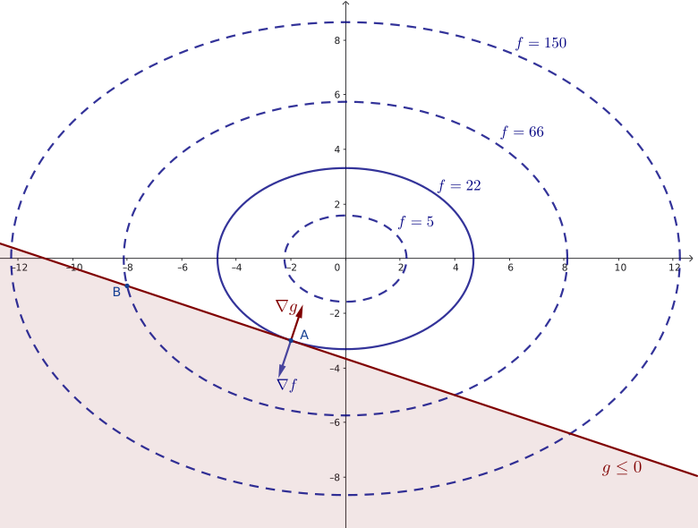
(A) $\nabla f \parallel \nabla g$ at the boundary w/ good directions
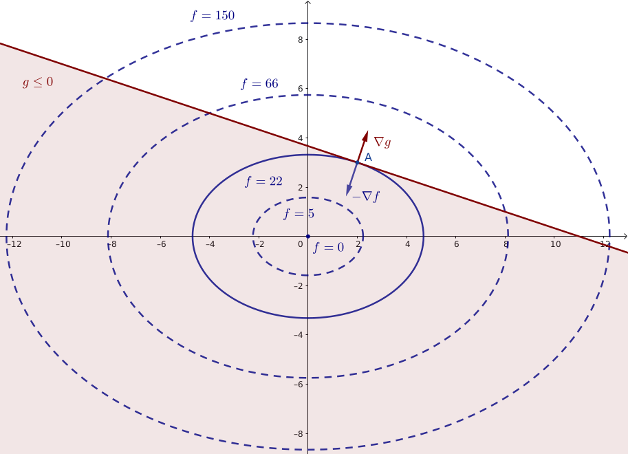
(B) $\nabla f \parallel \nabla g$ at the boundary but wrong directions
So the parallel condition itself is not sufficient. We need an additional requirement to distinguish the two subcases, and it is the direction. The feasible region is to the south west of the boundary. Let $\color{maroon}\nabla g$ point outwards, i.e. north east. Then $-\nabla f$, the descent direction, must also point outwards at the optimum. Otherwise, if $-\nabla f$ has any component that points into the region, we could move inwards and decrease $f$. That is, we need $\nabla f(\vec{x}^\ast) + \mu\nabla g(\vec{x}^\ast) = 0$ with $\mu\geq 0$.
KKT (Karush-Kuhn-Tucker) conditions
Case 1 also fits $\nabla f(\vec{x}^\ast) + \mu\nabla g(\vec{x}^\ast) = 0$, with $\mu = 0$. So in both cases, either $\mu = 0$ or $g(\vec{x}^\ast) = 0$, i.e. $\mu g(\vec{x}^\ast) = 0$. Putting everything together, consider the general problem
\[\begin{aligned} &\min f(\vec{x}) \\ \text{s.t. } &h_i(\vec{x}) = 0\ \forall i \\ &g_j(\vec{x}) \leq 0\ \forall j \end{aligned}\]. We minimise a multivariate function $f$, and we have $n$ equality constraints $h_1 = 0, \cdots, h_n = 0$, and $m$ inequality constraints $g_1\leq 0, \cdots, g_m\leq 0$. The Lagrangian is
\[\mathcal{L} = f + \sum_i\lambda_ih_i + \sum_j\mu_jg_j\]. The optimum must satisfy the KKT (Karush-Kuhn-Tucker) conditions:
\[\begin{align} \nabla_{\vec{x}}\mathcal{L}(\vec{x}^*) &= 0 \label{eq:stationary} \\ h_i(\vec{x}^*) &= 0 \label{eq:primal_1} \\ g_j(\vec{x}^*) &\leq 0 \label{eq:primal_2} \\ \mu_j &\geq 0 \label{eq:dual} \\ \mu_j g_j(\vec{x}^*) &= 0 \label{eq:complementary_slackness} \end{align}\]. Let’s go through them one by one.
Stationarity. ($\ref{eq:stationary}$) is the parallel condition, generalised to many constraints: $-\nabla f$ is a weighted sum of the constraint gradients.
Primal Feasibility. ($\ref{eq:primal_1}$) and ($\ref{eq:primal_2}$) require all constraints to be satisfied.
Dual Feasibility. The optimum happens at the boundary of, or inside the inequality constraints, so ($\ref{eq:dual}$) must hold.
Complementary Slackness. When the optimum is achieved at the boundary, $g$ has to be zero, and $\mu$ can be positive. When it’s inside the boundary, $\mu$ is then zero, because $g$ now is not active so we can remove it from the Lagrangian by setting $\mu$ to zero.
So just tell me how to solve it
In plain English, we solve a well behaved constrained optimisation in the following steps:1
- take the equality constraint only, and solve it. If we are lucky that this optimum also satisfies the inequality constraint, we are good
- if the above optimum violates the inequality constraint, then the actual optimum must happen on the boundary. Now treat the inequality constraint as if it’s equality, and solve again. Check the gradient directions at the optimum, i.e. $\mu\geq 0$. If it’s fine, we are good
It looks easy, but if we have multiple inequality constraints, things get combinatorially difficult: maybe the optimum happens on the boundary of inequality constraint 1 but inside inequality constraints 2 and 3. Or maybe on the boundary of 2 but inside 1 and 3, and so on. With $m$ inequality constraints, there are $2^m$ combinations of active and inactive constraints to check.
Physics interpretation
My favourite way to view KKT is through physics. Imagine we have a charged particle inside some electric field. It has some potential energy $f$, and naturally it wants to minimise the energy, i.e. $\min f$. The particle moves in a wire, and the shape of the wire is described by $h = 0$; it can’t leave the wire. The wire is not infinitely long, but bounded inside some area $g\leq 0$, e.g. some physical barrier like a wall or floor.
Stationarity. The electric force is $-\nabla f$, dragging the particle to lower its potential $f$. At equilibrium, this electric force is balanced by the force $\lambda\nabla h$ from the wire (to stop the particle from flying away) and the contact force $-\mu\nabla g$ from the barrier (if any, to stop the particle from going through the physical barrier). The three forces sum to zero, $-\nabla f - \lambda\nabla h - \mu\nabla g = 0$, which is exactly ($\ref{eq:stationary}$).
Dual Feasibility. $\mu$ must be zero (if the particle settles without touching the physical barrier), or positive (if the particle minimise its potential by pressing against the physical barrier).
Complementary Slackness. If the particle’s equilibrium is away from the barrier, then of course there is no contact force from the barrier. So $\mu$ is zero when $g$ is not zero.
When inequality constraint is not active
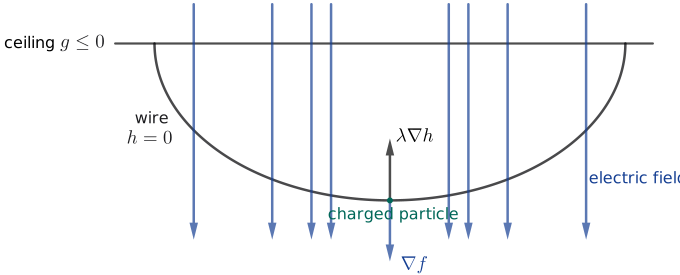
Imagine we have a wire hanging from the ceiling, and we have an electric field pointing down towards the floor. The wire is the equality constraint, and the ceiling is the inequality constraint (things can move below the ceiling but can’t break up through it). A charged particle gets minimal potential at the lowest point on the wire, where its electric force $\nabla f$ is balanced by the force from the wire $\lambda\nabla h$.2 The particle is not touching the ceiling, so it gets no force $\mu\nabla g$ from the ceiling, which implies $\mu = 0$.
When inequality constraint is active
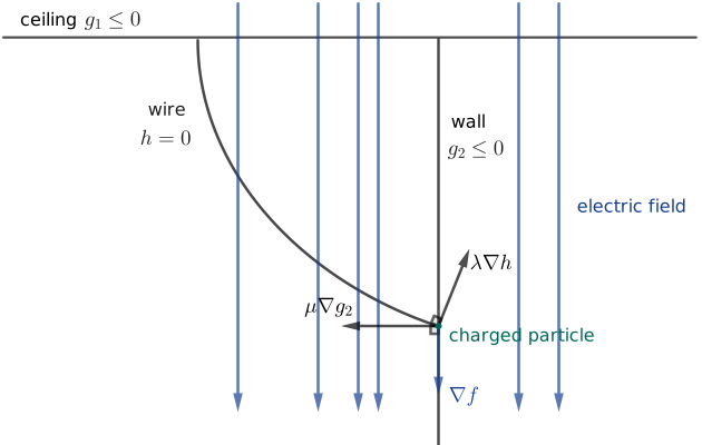
Now imagine another wire, hanging between the ceiling $g_1\leq 0$ and the wall $g_2\leq 0$. Again, the minimum potential happens at the lowest point on the wire. The particle gets the usual electric force $\nabla f$ and a force from the wire $\lambda\nabla h$, same as above. However, since it’s touching the wall, it gets one additional contact force $\mu_2\nabla g_2$ from the wall. The three forces are balanced in equilibrium, and now $\mu_2$ must be positive since the contact force is not zero. The particle is still not touching the ceiling, so $\mu_1 = 0$.
-
It needs to be a convex problem and meet a few regularity conditions. One example: $\min x$ s.t. $x^2\leq 0$. The only feasible point is $x = 0$, so it’s the optimum. But the stationary condition $\dfrac{\partial\mathcal{L}}{\partial x} = \dfrac{\partial (x + \mu x^2)}{\partial x} = 1 + 2\mu x = 1 + 0$ at the optimum. No $\mu$ can satisfy this, so stationary condition fails at optimum. Another example: $\max x$ s.t. $y - (1 - x)^3\leq 0, x\geq 0, y\geq 0$. We can show that the optimal point $(1, 0)$ doesn’t satisfy stationary condition either. In general, KKT is necessary under regularity conditions, and with convexity, it’s also sufficient. Without these nice properties, it’s neither necessary nor sufficient. See Farina (2025) for more discussions. ↩
-
It’s just to illustrate the idea. I may have missed a minus sign in front of these forces. ↩